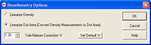
Selection of 'Options' from the Calibration window launches the following window.
Linearization of density is often appropriate as a basis for ICC profiling of color output with FM halftoning. This depends principally on the expectations of your ICC profiling software. For the production of color separation films, linearization of dot area is usually preferred. Many densitometers intended for the graphic arts provide a choice between measurement of density and measurement of dot area, but by using these controls, any densitometer can be used to linearize your choice of either dot area or density.
If you wish to linearize dot area instead of density, simply check it, and press "Set Default 'n'". Adjust away from the default setting if '1' if your specific situation demands it.
IMPORTANT - This tool converts density measurements into estimated dot area. Do not use this setting if you are already entering dot percent through "Hand Entry of Densitometry".
The software calculates dot area from density using the Murray-Davies/Yule-Nielsen equations that can be found in many technical books on color reproduction. The default setting of '1.0' for the Yule-Nielsen Correction 'n' reduces Yule-Nielsen to the Murray-Davies equation, and should be suitable for most linearization of films. A simplified version of the Murray-Davies equation is given in the notes below.
Linearizatin of dot area is usually chosen over linearization of density when producing color separation films with AM screens, like the AM screens used in the illustrations below.
The illustrations below show a linear PostScript gradient from zero to one hundred percent. They show how it will actually be printed after Wasatch SoftRIP as been linearized for dot area and after it has been linearized for density.
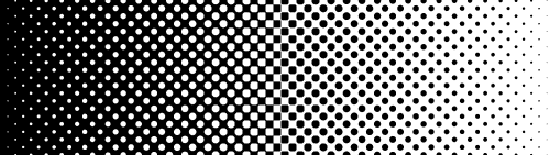
Linear Dot Area
The above illustration shows a halftoned gradient from zero to 100%. Notice that at the halfway point in this illustration, the halftone looks like a "checkerboard" in which dots cover half of the surface area. We call this point "50% dot", and because it appears in the exact middle of the above gradient, we say that the halftoned gradient is "linear" with respect to dot area.
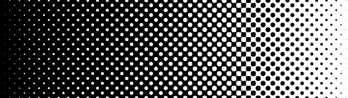
Linear Density
This illustration shows linear density where maximum density is 3.0. Together, these illustrations show that there is a big difference between linear dot and linear density. When density, instead of dot area, has been linearized, the "checkerboard" area moves a long distance away from the halfway point. When maximum density is greater than 3.0, this shift quickly becomes larger.
Here is why.The number reported by a densitometer as "density" has a "power of ten" relationship to the amount of light being blocked. When 99% of the light is blocked, the density is two. When 99.9% is blocked, density is three, 99.99% equates to a density of four, and so on. With reasonably dense films (films with a reaonably high dMmax), it is a good approximation to say that the amount of light being blocked is equal to the area covered by dots. The following formula is very close for this normal situation;
One over ten raised to the 'density' power equals the area not covered by dots
From high-school mathematics, one may recall that the inverse of this kind of exponential function is called a 'logarithm'. From this, we can also calulate what density will be for a given dot area.
density = -log(1.0 - dot area)
(These are simplfications. A more accurate solution is given by the Murray-Davies equations.)
For example where the dot area is 0.5 (50%), the density is 0.301, or about 30%. Density and dot are not the same thing at all, and more importantly, they are not linearly related.
The above illustration of "Linear Density" shows what will happen when linearizing density for film whose maximum density is 3.0. The "halfway point" has been mapped to a density of half of the maximum of 3.0, or 1.5, which causes the halfway point to be rendered with a dot area of about 70%. The shift becomes drastically more pronounced for films with maximum densities of more than 3.0.